|
1
|
- Conservation of Momentum
- Conservation of Mass
- Conservation of Energy
- Scaling Analysis
|
|
2
|
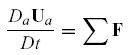
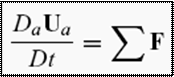
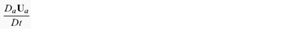
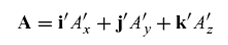
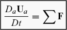
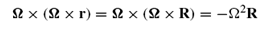
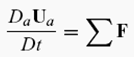
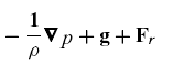
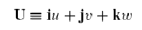
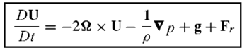
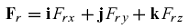
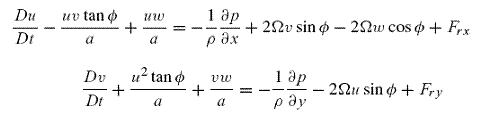
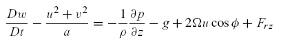
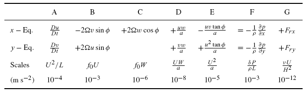
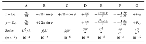
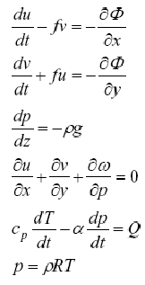
- The conservation law for momentum (Newton’s second law of motion)
relates the rate of change of the absolute momentum following the motion
in an inertial reference frame to the sum of the forces acting on the
fluid.
|
|
3
|
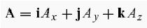
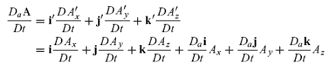
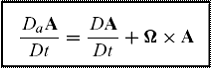
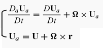
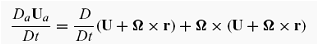
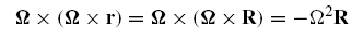
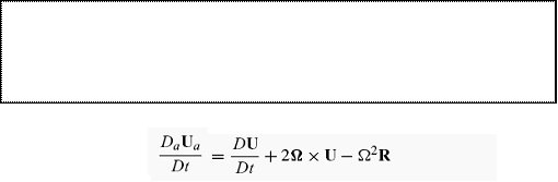
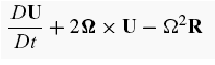
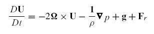
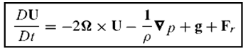
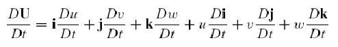
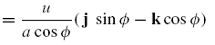
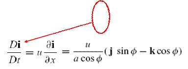
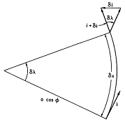
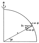
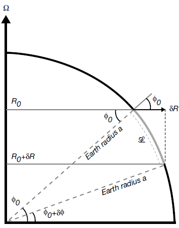
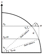
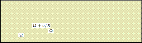
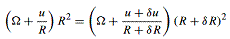
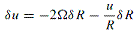
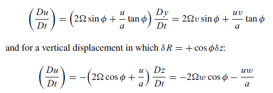
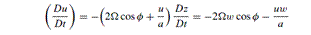
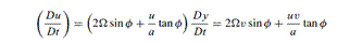
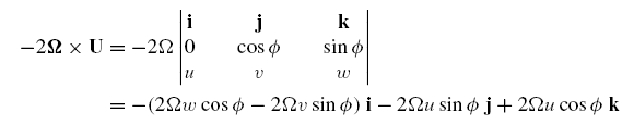
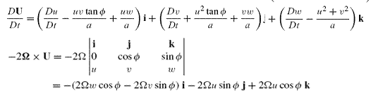
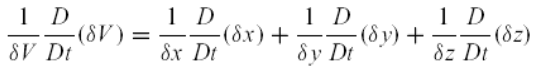
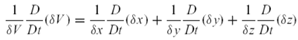
- For most applications in meteorology it is desirable to refer the motion
to a reference frame rotating with the earth.
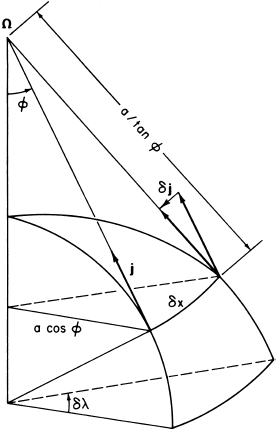
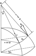
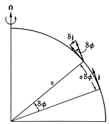
- Transformation of the momentum equation to a rotating coordinate system requires a
relationship between the total derivative of a vector in an inertial
reference frame and the corresponding total derivative in a rotating
system.
|
|
4
|
|
|
5
|
|
|
6
|
|
|
7
|
|
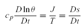
|
8
|
|
|
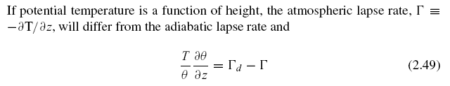
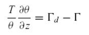
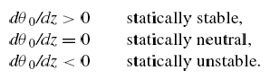
9
|
|
|
10
|
|
|
11
|
|
|
12
|
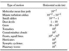
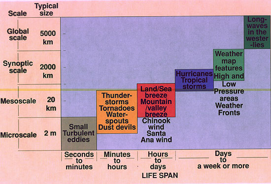
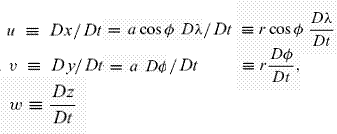
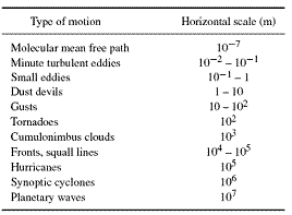
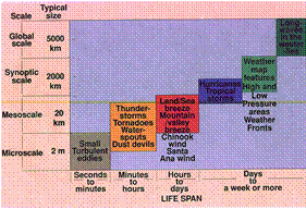
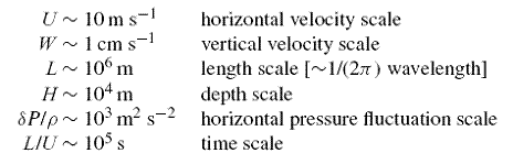
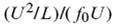
- Scale analysis, or scaling, is a convenient technique for estimating the
magnitudes of various terms in the governing equations for a particular
type of motion.
- In scaling, typical expected values of the following quantities are
specified:
- (1) magnitudes of the field
variables;
- (2) amplitudes of
fluctuations in the field variables;
- (3) the characteristic
length, depth, and time scales on which these fluctuations occur.
- These typical values are then used to compare the magnitudes of various
terms in the governing equations.
|
|
13
|
|
|
14
|
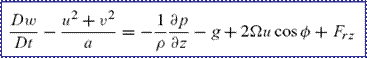
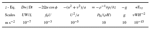
- The complete set of the momentum equations describe all scales of
atmospheric motions.
- We need to simplify the equation for synoptic-scale motions.
- We need to use the following characteristic scales of the field
variables for mid-latitude synoptic systems:
|
|
15
|
- Pressure Gradients
- The pressure gradient force initiates movement of atmospheric mass,
wind, from areas of higher to areas of lower pressure
- Horizontal Pressure Gradients
- Typically only small gradients exist across large spatial scales
(1mb/100km)
- Smaller scale weather features, such as hurricanes and tornadoes,
display larger pressure gradients across small areas (1mb/6km)
- Vertical Pressure Gradients
- Average vertical pressure gradients are usually greater than extreme
examples of horizontal pressure gradients as pressure always decreases
with altitude (1mb/10m)
|
|
16
|
|
|
17
|
|
|
18
|
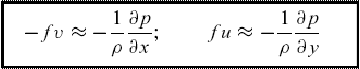
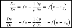
- In order to obtain prediction equations, it is necessary to retain the
acceleration term in the momentum equations.
- The geostrophic balance make the weather prognosis (prediction)
difficult because acceleration is given by the small difference between
two large terms.
- A small error in measurement of either velocity or pressure gradient
will lead to very large errors in estimating the acceleration.
|
|
19
|
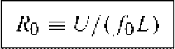
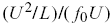
- Rossby number is a non-dimensional measure of the magnitude of the
acceleration compared to the Coriolis force:
- The smaller the Rossby number, the better the geostrophic balance can be
used.
- Rossby number measure the relative importnace of the inertial term and
the Coriolis term.
- This number is about O(0.1) for
Synoptic weather and about O(1) for ocean.
|
|
20
|
|
|
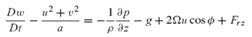
21
|
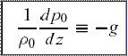
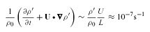
- The acceleration term is several orders smaller than the hydrostatic
balance terms.
- è Therefore,
for synoptic scale motions, vertical accelerations are negligible and
the vertical velocity cannot be determined from the vertical momentum
equation.
|
|
22
|
- For synoptic-scale motions, the vertical velocity component is typically
of the order of a few centimeters per second. Routine meteorological
soundings, however, only give the wind speed to an accuracy of about a
meter per second.
- Thus, in general the vertical velocity is not measured directly but must
be inferred from the fields that are measured directly.
- Two commonly used methods for inferring the vertical motion field are
(1) the kinematic method, based on the equation of continuity, and (2)
the adiabatic method, based on the thermodynamic energy equation.
|
|
23
|
|
|
24
|
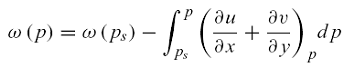
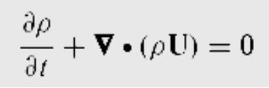
- We can integrate the continuity equation in the vertical to get the
vertical velocity.
|
|
25
|
- The adiabatic method is not so sensitive to errors in the measured
horizontal velocities, is based on the thermodynamic energy equation.
|
|
26
|
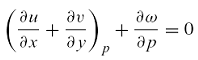
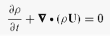
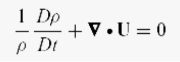
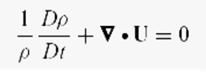
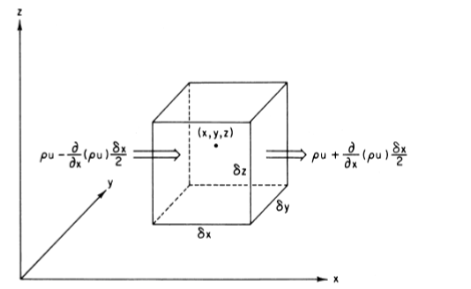
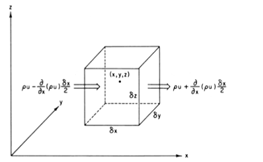
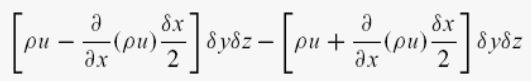
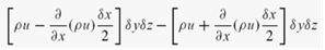
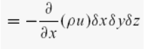
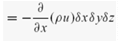
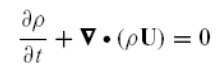
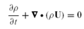
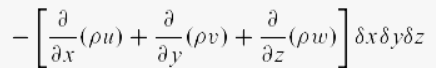
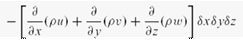
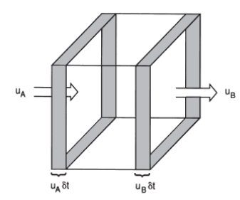
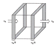
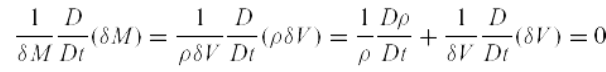
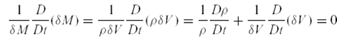
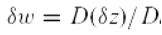
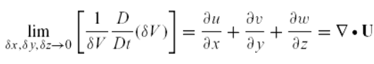
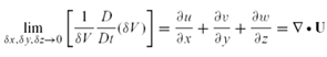
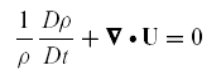
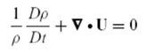
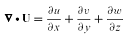
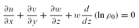
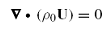
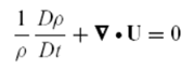
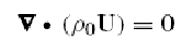
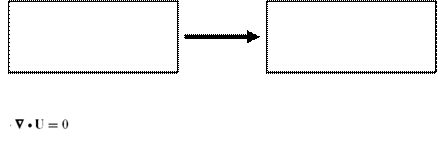
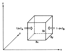
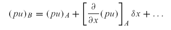
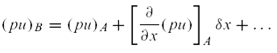
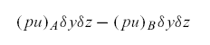
- The mathematical relationship that expresses conservation of mass for a
fluid is called the continuity equation.
|
|
27
|
|
|
28
|
|
|
29
|
|
|
30
|
|
|
31
|
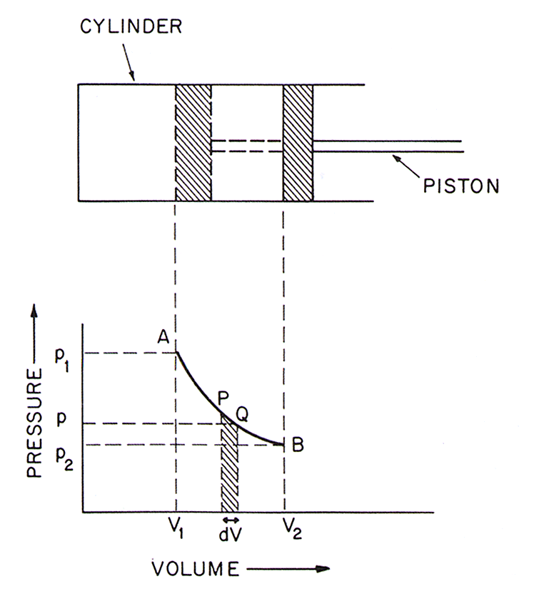
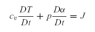
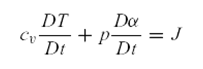
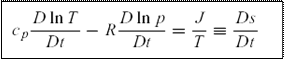
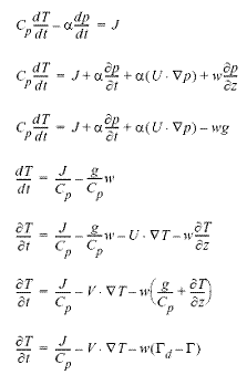
- This law states that (1) heat is a form of energy that (2) its
conversion into other forms of energy is such that total energy is
conserved.
- The change in the internal energy of a system is equal to the heat added
to the system minus the work down by the system:
|
|
32
|
- Therefore, when heat is added to a gas, there will be some combination
of an expansion of the gas (i.e. the work) and an increase in its
temperature (i.e. the increase in internal energy):
|
|
33
|
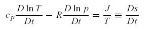
- Heat and temperature are both related to the internal kinetic energy of
air molecules, and therefore can be related to each other in the
following way:
|
|
34
|
|
|
35
|
- The first law of thermodynamics is usually derived by considering a
system in thermodynamic equilibrium, that is, a system that is initially
at rest and after exchanging heat with its surroundings and doing work
on the surroundings is again at rest.
- A Lagrangian control volume consisting of a specified mass of fluid may
be regarded as a thermodynamic system. However, unless the fluid is at
rest, it will not be in thermodynamic equilibrium. Nevertheless, the
first law of thermodynamics still applies.
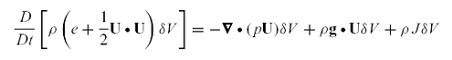
- The thermodynamic energy of the control volume is considered to consist
of the sum of the internal energy (due to the kinetic energy of the
individual molecules) and the kinetic energy due to the macroscopic
motion of the fluid. The rate of change of this total thermodynamic
energy is equal to the rate of diabatic heating plus the rate at which
work is done on the fluid parcel by external forces.
|
|
36
|
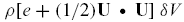
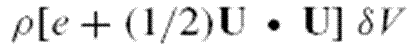
- If we let e designate the internal energy per unit mass, then the total
thermodynamic energy contained in a Lagrangian fluid element of density ρ
and volume δV is
|
|
37
|
- The external forces that act on a fluid element may be divided into
surface forces, such as pressure and viscosity, and body forces, such as
gravity or the Coriolis force.
- However, because the Coriolis force is perpendicular to the velocity
vector, it can do no work.
|
|
38
|
|
|
39
|
|
|
40
|
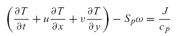
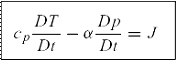
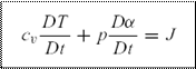
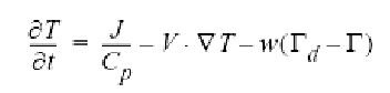
- After many derivations, this is the usual form of the thermodynamic
energy equation.
- The second term on the left, representing the rate of working by the
fluid system (per unit mass), represents a conversion between thermal
and mechanical energy.
- This conversion process enables the solar heat energy to drive the
motions of the atmosphere.
|
|
41
|
|
|
42
|
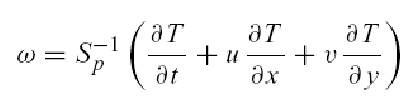
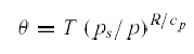
- For an ideal gas undergoing an adiabatic
process (i.e., a reversible process in which no heat is exchanged
with the surroundings; J=0), the first law of thermodynamics can be
written in differential form as:
|
|
43
|
|
|
44
|
|
|
45
|
- Pressure Gradients
- The pressure gradient force initiates movement of atmospheric mass,
wind, from areas of higher to areas of lower pressure
- Horizontal Pressure Gradients
- Typically only small gradients exist across large spatial scales
(1mb/100km)
- Smaller scale weather features, such as hurricanes and tornadoes,
display larger pressure gradients across small areas (1mb/6km)
- Vertical Pressure Gradients
- Average vertical pressure gradients are usually greater than extreme
examples of horizontal pressure gradients as pressure always decreases
with altitude (1mb/10m)
|
|
46
|
|
|
47
|
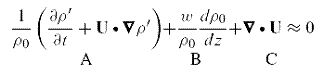
- Term A: Diabatic Heating
- Term B: Horizontal Advection
- Term C: Adiabatic Effects
|
|
48
|
- The scaling analyses results in a set of approximate equations that
describe the conservation of momentum, mass, and energy for the
atmosphere.
- These sets of equations are called the primitive equations, which are
very close to the original equations are used for numerical weather
prediction.
- The primitive equations does not describe the moist process and are for
a dry atmosphere.
|
|
49
|
|

 Notes
Notes