Discussion

From Figures 6.28 and 6.29, it is clear that enhanced levels of BrO are present. What is surprising, however, is the horizontal extent of this enhancement. Long periods of sustained enhancement were observed over the middle portion of each flight in which the ER-2 was either over the Arctic Ocean or the Queen Elizabeth Islands, NWT. There was also larger variability towards the beginning and end of each flight. Analysis of a third flight made on 13 May 1997 produced BrO mixing ratios similar in size and spatial extent to that from the 2 May and 6 May flights. These observations are consistent with the suggestion that the bromine source is sea-salt particles originating from leads in the sea ice, as suggested by McConnell et al. (1992). During the 6 May flight, mixing ratios of larger than 10 pptv were observed from 73-84 ksec during which time the ER-2 travelled about 2300 km. The exception to this was during a 5 ksec stretch at the end of the 2 May flight, about 1000 km, in which mixing ratios steadily increased up to 40 pptv. The last hour of this flight was also well inland, up to 600 km from the nearest shore.

The large spatial extent of the enhanced BrO implies that a large amount of ozone is being destroyed. The ozone loss rate can be expressed approximately as,

$$\frac{d[{\rm O_3}]}{dt} = - 2 k [{\rm BrO}]^2$$ (11.49)

where $k=4\times10^{-12}$ cm³ s^-1 is the reaction rate coefficient for equation (6.39), the rate limiting step, and $[{\rm O_3}]$ and $[{\rm BrO}]$ are the ozone and BrO number densities, respectively. Note that ozone loss rate, equation (6.49), is independent of the ozone concentration which is valid as long as there is at least 1 ppbv of ozone present. For 15 pptv of BrO at the surface in the Arctic, $[{\rm BrO}]=4.1\times 10^8$ cm^-3, and the ozone loss rate is 4.3 ppbv/day. If the bulk of BrO persists from 2 to 13 May, then much of the PBL ozone in this regions will be destroyed. Continued depletion over an even longer period could impact the overall Arctic tropospheric ozone budget.

 

Global Ozone Monitoring Experiment (GOME) BrO VCDs for selected three day averages throughout spring 1997 are presented in Figure 6.31 (Richter et al., 1998). They were calculated by choosing the reference spectra to be from the longitude band which gave the lowest ACDs from the same three day period and thus represent a lower limit of the excess BrO VCD (Richter et al., 1998). As is evident by comparing the GOME VCDs to those from panel (e) in Figures 6.28 and 6.29, the results are of similar magnitude. The GOME excess VCDs are observed to be 4-7 $\times 10^{13}$ cm^-2 over much of the North American Arctic throughout the entire spring. A maximum VCD of $1.5\times 10^{14}$ cm^-2 occurred in early March (A. Richter, personal communication, 1998). Placing these GOME excess BrO VCDs inside a 1 km PBL results in mixing ratios of 16-28 pptv, with a maximum of 60 pptv. This latter value is reminiscent of results from the 26 April flight (discussed below). The horizontal extent of the excess BrO is very large, larger even than was observed from the ER-2. At its peak in March and April, excess BrO is present over an area in excess of $5\times 10^6$ km². Similar to the arguments made when considering the CPFM measurements, sustaining these levels of BrO over this long a period must result in a large amount of ozone destruction.

As mentioned previously, Arctic PBL heights as inferred from temperature soundings in April and May 1997 were 0.3-0.8 km and so the adopted value of 1 km represents an upper limit. Thus, the BrO mixing ratios quoted above are likely a lower limit. For the shallowest of PBLs, values could increase by a factor of three, large enough that it is reasonable to expect that some fraction of the excess BrO is present in the free troposphere.

If conclusions concerning the location (PBL or free troposphere) of the enhanced BrO for the May ER-2 flights and the GOME measurements are dependent upon the height of the PBL, the PBL height is not an issue for the results of the 26 April flight. Until now, it was generally accepted that the enhanced levels of BrO and other bromine species are present only within the PBL, and at levels not exceeding 40-50 pptv. However, from the results of the 26 April flight, one of these assumptions cannot be true. As the maximum total bromine in the PBL has been measured to be approximately 100 pptv (Berg et al., 1982), by assuming all of the observed BrO was present in the PBL, all the PBL bromine would have to be in the form of BrO. The more feasible alternative is that a significant fraction the BrO must reside above the PBL in the free troposphere. Recent measurements made at Kangerlussuaq, Greenland (Miller et al., 1997) and in the Antarctic (Kreker et al., 1997) also suggested that enhanced amounts of BrO may reside higher in the atmosphere, although in each case it was not possible to ascertain where.

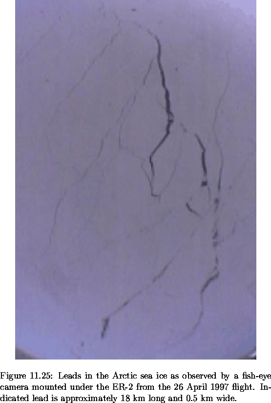
Having suggested that a substantial fraction of the BrO measured on 26 April was present in the free troposphere, a number of questions must be answered. First and foremost: how did it get there? The most abundant form of bromine already present in the free troposphere is CH₃Br, present at 10-15 pptv (WMO, 1995). This can be converted to BrO via reactions with OH but this reaction sequence is very slow. A more likely source is transport of PBL BrO into the free troposphere. One possible mechanism is convection, generated by large temperature contrasts between the ambient air and the warmer water, over open leads in the Arctic sea ice. These buoyant plumes of air may be lofted as high as 3 to 4 km, well above the top of the PBL (Andreas et al., 1990; Schnell et al., 1989). Modeling studies suggest that for convection to these altitudes, open leads must be about 10 km wide. These are likely to be rare, although semipermanent shore leads can frequently be this wide (Serreze et al., 1992). Plumes from leads this large have been observed over 200 km downwind from their surface source (Andreas et al., 1990). A still frame of leads in the sea ice, made by a fish-eye camera installed on the bottom of the ER-2 during the 26 April flight, is shown in Figure 6.32. The lead, running north to south in the upper half of the photograph, is approximately 18 km long and 0.5 km wide. It cannot be determined from this if the lead is open or closed. Also, leads much larger than this would be necessary to produce enough convection to loft air up to 4 km.

 

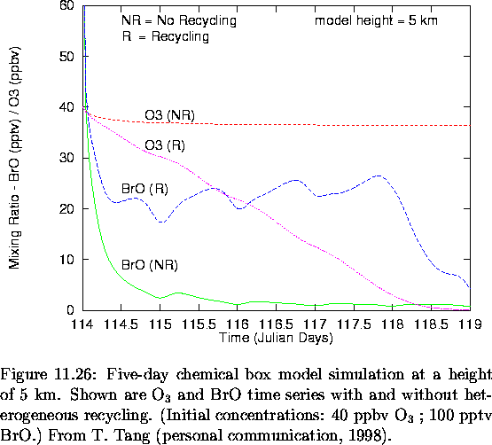
As the BrO was observed in the free troposphere throughout the 7-hour flight, another question is how can these levels of BrO remain for time periods on the order of 1 day? Results from a chemical box model (chemistry at a point) simulation, using the model of Tang and McConnell (1996), are presented in Figure 6.33 (T. Tang, personal communication, 1998). The model height was 5 km for this simulation and it was run with and without BrO recycling. It is assumed that all bromine is initially present as BrO but the model chemistry rapidly repartitions the bromine.

 

From Figure 6.33 it is clear that without recycling the lifetime of Br+BrO is about 6 hours. Hence, over the course of the flight, with no heterogeneous chemistry, the BrO would have been reduced by over a factor of three, which was not observed. Therefore, heterogeneous chemistry, through reactions similar to that in equation (6.46), must be converting HBr back to BrO. With recycling, the BrO was maintained at 20 pptv for about four days. Also, even with recycling the lifetime of the ozone was about three days. The ozone loss rate in terms of mixing ratio, from equation (6.49), is proportional to the background air number density. For equal BrO mixing ratios at the surface and 5 km, the ozone destruction rate will be reduced by a factor of two at 5 km from that at the surface as the pressure has dropped by a factor of two. With the reduced destruction rate and the increased mixing in the free troposphere between the ozone-rich and ozone-depleted air, it would be hard to detect an ozone depletion signature.

A number of surfaces are available in the free troposphere on which heterogeneous chemistry can take place. Tropospheric sulphates are ubiquitous and have been measured by Parungo et al. (1993) and others. Additionally, ice crystals and water droplets in the PBL may be transported in the same manner as the BrO: through convection over large open leads in the sea ice. Ice crystals in the lower troposphere have been suggested previously as heterogeneous chemistry sites to explain the rapid ozone destruction (Curry and Radke, 1993). Supercooled water droplets contained within these plumes with concentrations on the order of 1 cm^-3 have been observed by airborne lidar (Schnell et al., 1989).

Further support for the argument that, in general, some of the enhanced PBL BrO must be transported into the free troposphere can be inferred from the GOME measurements. From Figure 6.31, enhanced levels of BrO are present for over three months over the Arctic Ocean and NWT. Mixing with air from the free troposphere will occur with the break up of the inversion layer (for example, during a storm) and so on this basis, some BrO must be transported into the free troposphere. The fact that during March and April elevated BrO is observed over the NWT up to 1000 km inland suggests that the heterogeneous mechanism is not restricted to the marine environment, and hence not necessarily restricted to the PBL either.

The homogeneity (or lack thereof) of the PBL height throughout the Arctic will also influence conclusions concerning the horizontal uniformity of the enhanced BrO. For example, if the PBL height varies on a horizontal scale of 100 km, the variability observed in the VCDs over the three flights might be largely the result of a PBL of variable height and constant BrO mixing ratio.

   

Figure 6.35: As Figure 6.34 but for ozone profiles.

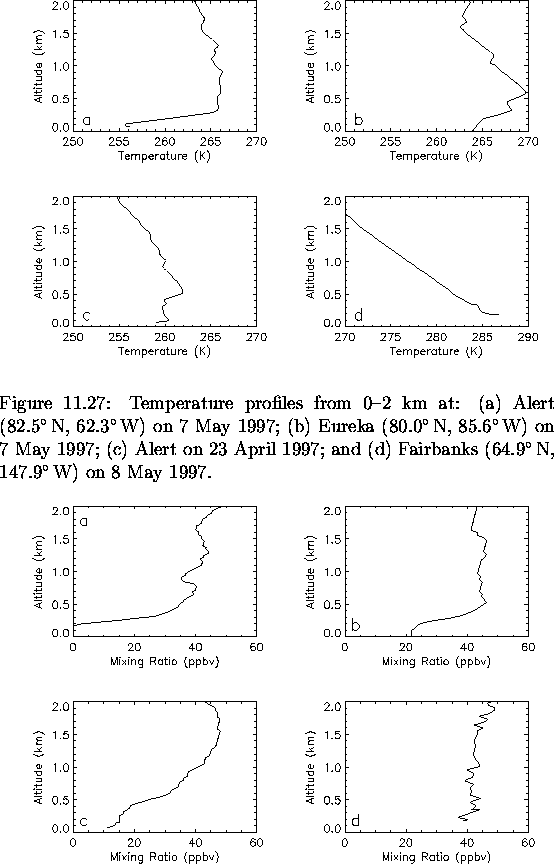
Finally, to further illustrate the polar sunrise ozone depletion phenomena, four sample ozonesonde measurements are presented. Figures 6.34 and 6.35 show temperature and ozone profiles, respectively, from 0-2 km for four ozonesondes launched in the Arctic between 23 April and 8 May 1997. Each was launched around noon local time and was aloft for approximately 2-3 hours. Panel (a) in both figures corresponds to a well defined PBL and near zero O₃ levels within. Note the late date of this depletion event: a week into May, generally later than expected. From panel (b), a temperature inversion is also present and there is evidence for O₃ destruction as levels have been reduced to half of the background. The temperature profile from panel (c) indicates that the PBL is stable even through there is no temperature inversion and from the ozone profile significant ozone depletion is observed up to 1 km. Panel (d) is an example of no temperature inversion and no O₃ depletion. The PBL heights of the two temperature profiles which displayed obvious temperature inversions were 0.3 km and 0.6 km.