Based on the results of the sensitivity study described
above, an aerosol retrieval algorithm was developed.
As a guide to which quantities may be retrieved, recall
that in the visible the absolute uncertainty in the radiance is
estimated at 10%. Similarly, the uncertainty in the polarization is
estimated at 0.03.
Again, quantities are deemed potentially retrievable if the radiance or
polarization were observed to vary by at least these amounts
over the expected range for this quantity.
For example, polarization did not change by 0.03 over the range
of refractive indices expected for stratospheric aerosols and
so refractive index is not a good candidate for retrieval.
Further, attention will be restricted
to stratospheric aerosols and so only elevation angles which do
not probe into the troposphere are considered. This excludes
EAs below
![]() .
.
A summary of the sensitivity results is given in Table 5.5 where the
degree to which a given parameter can be retrieved has been estimated.
Both radiance and polarization were found to be sensitive to both the amount
and the height of the aerosol number density, indicating that the
retrieval of a vertical profile of the extinction coefficient is possible.
When examining the size parameters, radiance was found to be largely
insensitive while polarization was sensitive to the effective radius and
effective variance (the latter only for
![]() ).
This suggests polarization can be used to retrieve size information.
Refractive index had a very small impact on radiance and moderate
impact on polarization. Over the range expected in the stratosphere,
1.39-1.46, less than a 0.02 variation in polarization was found.
This suggests that refractive index can not be retrieved to better than
0.07. Finally, neither radiance nor polarization can be used to
determine the vertical variation of effective radius.
The range in scaling factors used was fairly restrictive
(
).
This suggests polarization can be used to retrieve size information.
Refractive index had a very small impact on radiance and moderate
impact on polarization. Over the range expected in the stratosphere,
1.39-1.46, less than a 0.02 variation in polarization was found.
This suggests that refractive index can not be retrieved to better than
0.07. Finally, neither radiance nor polarization can be used to
determine the vertical variation of effective radius.
The range in scaling factors used was fairly restrictive
(![]() )
and in many cases the aerosol amounts exceed those
of the standard background profile by factors of 2-5, such as
after a recent volcanic eruption. Under these conditions, the
Mie scattering signal should increase but it is difficult to
determine by how much without further model calculations.
)
and in many cases the aerosol amounts exceed those
of the standard background profile by factors of 2-5, such as
after a recent volcanic eruption. Under these conditions, the
Mie scattering signal should increase but it is difficult to
determine by how much without further model calculations.
a For ideal geometry, 0.05
|
To simplify the retrieval process, it is broken down into
two parts; extinction coefficient profiles and size distribution
are determined separately. As radiance was observed to be
sensitive to the amount of aerosol but less sensitive to the size parameters
for a given optical depth, it is used to first determine
the extinction coefficient profile. However, as only 6-8 steps
in a scan will be used and with the information contained in each
not independent of the others, it will not be possible to obtain
a detailed profile. Despite this, the main characteristics can be captured
by supplementing the information from the measurements with
a priori knowledge. McCormick et al. (1996) has suggested
that the stratospheric extinction coefficient profiles are well
represented by,
| (9.9) |
Once the extinction coefficient profile is known, the polarization data
can be used to obtain the effective radius and effective variance.
Values of
![]() and
and
![]() are determined by varying
them, using a log-normal size distribution,
until the model polarization matches the measurements.
Again a wavelength of 750 nm is used. As the limb radiance was
not totally insensitive to the effective radius (maximum difference
of 30% between 0.10 and 0.30
are determined by varying
them, using a log-normal size distribution,
until the model polarization matches the measurements.
Again a wavelength of 750 nm is used. As the limb radiance was
not totally insensitive to the effective radius (maximum difference
of 30% between 0.10 and 0.30 ![]() m), the first step should be
performed again using the estimated values of
m), the first step should be
performed again using the estimated values of
![]() and
and
![]() .
If there is a substiantial change in the
values of
.
If there is a substiantial change in the
values of
![]() -
-
![]() ,
the second step should also
be repeated.
It is estimated that two iterations should be sufficient.
,
the second step should also
be repeated.
It is estimated that two iterations should be sufficient.
Once the size distribution is known, Mie cross-sections can be computed
to obtain a number density profile,
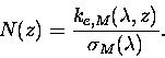 |
(9.10) |
Comparisons can be made with two in-situ instruments
also flown on the ER-2.
The first is the ER-2 Condensation Nucleus Counter (CNC) II which counts
particles with radii between 0.004 and 1 ![]() m (Wilson et al., 1983).
The second is the Focused Cavity Aerosol Spectrometer (FCAS) II
which also detects particles over this same range
(Jonsson et al., 1995).
The FCAS II also measures aerosol surface area per unit
volume and aerosol volume per unit volume. For comparison with
retrieved aerosol densities at ER-2 height, the surface area
and volume densities for the log-normal size distribution can be computed,
m (Wilson et al., 1983).
The second is the Focused Cavity Aerosol Spectrometer (FCAS) II
which also detects particles over this same range
(Jonsson et al., 1995).
The FCAS II also measures aerosol surface area per unit
volume and aerosol volume per unit volume. For comparison with
retrieved aerosol densities at ER-2 height, the surface area
and volume densities for the log-normal size distribution can be computed,
| SA(z) | = | 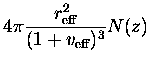 |
(9.11) |
| V(z) | = | 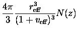 |
(9.12) |
This algorithm was applied to limb scans from two flights made as part of the POLARIS campaign. The algorithm and retrieved aerosol properties are described in an article entitled ``Observations of stratospheric aerosols using CPFM polarized limb radiances'' accepted for publication in the Journal of the Atmospheric Sciences in January 1998. A copy of this paper is given in Appendix C.