The method used in this study to solve the equation of radiative transfer is the successive orders of scattering technique. It was chosen for two main reasons; 1) it is physically intuitive, especially as the physics remains clear through the mathematical formalism, and hence relatively easy to code; and 2) it is easily adaptable to different geometries and types of simulations.
The equation of radiative transfer may be obtained from the Boltzmann
transport equation for photons where it is assumed that interactions
between photons can be ignored.
For an inhomogeneous scattering atmosphere, the general
equation of radiative transfer without specifying any coordinate system is,
| (3.71) |
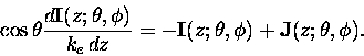
The last term on the right hand side of equation (2.70) is called the source function vector. The first term on the right hand side represents attenuation due to absorption and scattering of a radiance stream as it propagates through the atmosphere, and the source function vector represents the strengthening of the radiance stream. For solar radiation it arises from photons scattered in the path from all other directions. The presence of this scattering source term ensures that the radiation field is no longer merely a function of local sources and sinks, but of the entire atmospheric radiation field and of its transport over large distances. In practice this makes the solution much more difficult to obtain.
The radiance field can be taken as time independent or in a steady
state so that
![]() .
Also, only elastic scattering is considered.
To simplify the solution further,
the atmosphere is approximated as being vertically stratified and
horizontally homogeneous. This reduces the number of spatial dimensions
from three to one, with the solution a function of height only. The
position vector
.
Also, only elastic scattering is considered.
To simplify the solution further,
the atmosphere is approximated as being vertically stratified and
horizontally homogeneous. This reduces the number of spatial dimensions
from three to one, with the solution a function of height only. The
position vector ![]() is replaced by the scalar z.
This is called plane parallel geometry. The natural plane-parallel
co-ordinates are the spherical polar angles
is replaced by the scalar z.
This is called plane parallel geometry. The natural plane-parallel
co-ordinates are the spherical polar angles ![]() and
and ![]() which replace the the directional unit vector,
which replace the the directional unit vector,
![]() .
Taking all this into account, equation (2.70) can be
simplified to,
.
Taking all this into account, equation (2.70) can be
simplified to,
It will prove convenient to introduce an alternative vertical coordinate
which takes into effect the optical properties of the atmosphere and which
is also
independent of the physical distance. The optical depth is defined as,
The scattering angle ![]() can be represented in terms of the
direction of the incident radiation (
can be represented in terms of the
direction of the incident radiation (
![]() )
and the direction of
the scattered radiation (
)
and the direction of
the scattered radiation (![]() ),
),
| (3.75) |
The multiple scattering source function vector can be expressed as,
| = | 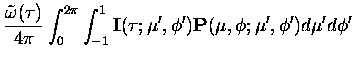 |
||
 |
(3.76) |
 |
(3.77) |
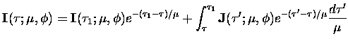
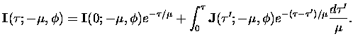
Equation (2.74) can be recast into integral form
by introducing integrating factors. For the downward streams,
the factor
![]() is used while for upward streams,
is used while for upward streams,
![]() is used. The result is,
is used. The result is,
| (3.80) |
Solution to equation (2.74) will only give the scattered,
or diffuse, radiation field; the direct, or unscattered, component must be
added separately.
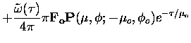
The total (direct+diffuse) downward radiance is given by,
| (3.81) |